R and Deep Learning CNN for Handwritten Digits Recognition

The MNIST database consists of handwritten digits. The training set has 60,000 examples, and the test set has 10,000 examples. The MNIST database is a subset of a larger set available from NIST. The digits have been size-normalized and centered in a fixed-size image. The original NIST’s training dataset was taken from American Census Bureau employees, while the testing dataset was taken from American high school students. For MNIST dataset, half of the training set and half of the test set were taken from NIST’s training dataset, while the other half of the training set and the other half of the test set were taken from NIST’s testing dataset.

For the MNIST dataset, the original black and white (bilevel) images from NIST were size normalized to fit in a 20×20 pixel box while preserving their aspect ratio. The resulting images contain grey levels as a result of the anti-aliasing technique used by the normalization algorithm. the images were centered in a 28×28 image (for a total of 784 pixels in total) by computing the center of mass of the pixels, and translating the image so as to position this point at the center of the 28×28 field.

Deep learning is still fairly new to R. The main purpose of this blog is to conduct experiment to get myself familiar with the ‘h2o’ package. As we are know, there many machine learning R packages such as decision tree, random forest, support vector machine etc. The creator of the h2o package has indicted that h2o is designed to be “The Open Source In-Memory, Prediction Engine for Big Data Science”.

Step 1: Load the training dataset

In this experiment, the Kaggle pre-processed training and testing dataset were used. The training dataset, (train.csv), has 42000 rows and 785 columns. The first column, called “label”, is the digit that was drawn by the user. The rest of the columns contain the pixel-values of the associated image.

Each pixel column in the training set has a name like pixelx, where x is an integer between 0 and 783, inclusive. To locate this pixel on the image, suppose that we have decomposed x as x = i * 28 + j, where i and j are integers between 0 and 27, inclusive. Then pixelx is located on row i and column j of a 28 x 28 matrix, (indexing by zero).

train <- read.csv ( "train.csv")

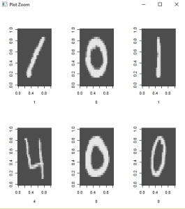
The hand written images are rotated to the left. In order to view some of the images, rotations to the right will be required.

# Create a 28*28 matrix with pixel color values
m = matrix(unlist(train[10,-1]), nrow = 28, byrow = TRUE)

# Plot that matrix
image(m,col=grey.colors(255))

# reverses (rotates the matrix)
rotate <- function(x) t(apply(x, 2, rev)) 

# Plot some of images
par(mfrow=c(2,3))
lapply(1:6, 
       function(x) image(
         rotate(matrix(unlist(train[x,-1]),nrow = 28, byrow = TRUE)),
         col=grey.colors(255),
         xlab=train[x,1]
       )
)

par(mfrow=c(1,1)) # set plot options back to default

Step 2: Separate the dataset to 80% for training and 20% for testing

Using the caret package, separate the train dataset. Store the training and testing datasets into separate .csv files.

library (caret)
inTrain<- createDataPartition(train$label, p=0.8, list=FALSE)
training<-train.data[inTrain,]
testing<-train.data[-inTrain,]

#store the datasets into .csv files
write.csv (training , file = "train-data.csv", row.names = FALSE) 
write.csv (testing , file = "test-data.csv", row.names = FALSE)

Step 3: Load the h2o package

library(h2o)

#start a local h2o cluster
local.h2o <- h2o.init(ip = "localhost", port = 54321, startH2O = TRUE, nthreads=-1)

Load the training and testing datasets and convert the label to digit factor

training <- read.csv ("train-data.csv") 
testing  <- read.csv ("test-data.csv")

 # convert digit labels to factor for classification
training[,1]<-as.factor(training[,1])

# pass dataframe from inside of the R environment to the H2O instance
trData<-as.h2o(training)
tsData<-as.h2o(testing)

Step 4: Train the model

Next is to train the model. For this experiment, 5 layers of 160 nodes each are used. The rectifier used is Tanh and number of epochs is 20

res.dl <- h2o.deeplearning(x = 2:785, y = 1, trData, activation = "Tanh", hidden=rep(160,5),epochs = 20)

Step 5: Use the model to predict

#use model to predict testing dataset
pred.dl<-h2o.predict(object=res.dl, newdata=tsData[,-1])
pred.dl.df<-as.data.frame(pred.dl)

summary(pred.dl)
test_labels<-testing[,1]

#calculate number of correct prediction
sum(diag(table(test_labels,pred.dl.df[,1])))

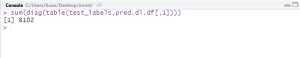
From the model, the accuracy of prediction for the testing dataset is 96.48% (8102 out of 8398).

Step 6: Predict test.csv and submit to Kaggle

Lastly, use the model to predict test.csv and submit the result to Kaggle.

# read test.csv
test<-read.csv("test.csv")

test_h2o<-as.h2o(test)

# convert H2O format into data frame and save as csv
df.test <- as.data.frame(pred.dl.test)
df.test <- data.frame(ImageId = seq(1,length(df.test$predict)), Label = df.test$predict)
write.csv(df.test, file = "submission.csv", row.names=FALSE)

# shut down virtual H2O cluster
h2o.shutdown(prompt = FALSE)

Result from Kaggle shows the accuracy of 96.514%.